
The obvious way to build a photo culling tool in 2026 is to throw a vision-language model at it. Feed each image to a VLM, ask “is this a good photo?”, parse the answer. It works — at maybe one image every few seconds, a couple of gigabytes of weights resident, and a verdict you can’t audit because it’s a single probability from a black box. On an 8 GB MacBook Air with a real photo library, it’s a non-starter.
SnapGrade is the bet that classical computer vision, applied carefully, covers what actually makes a photo a keeper or a reject. Blur, closed eyes, blown highlights, burst duplicates, horizon tilt — each has a precise, fast, interpretable measure. No transformer required. The pipeline runs at 3.3 images per second on the same 8 GB machine, re-runs are instant (SQLite cache), and every verdict comes with a human-readable reason string instead of a confidence score.
This post walks through the architecture, the metric stack, the threshold-based decision layer, and the optimization work that took throughput from 1.9 to 3.3 img/s.
Three Layers That Share Nothing but SQLite
The system has three layers that share no state except the database:
flowchart TD
    subgraph "Analyzer (pure image → metrics)"
        A[Image Decode\ndecode.py] --> B[EXIF Extraction\nexif.py]
        A --> C[Sharpness\nLaplacian + Tenengrad + FFT]
        A --> D[Subject Detection\nMediaPipe face + saliency]
        A --> E[Blink Detection\nFaceMesh + EAR]
        A --> F[Exposure\nhistogram + clipping]
        A --> G[Perceptual Hash\npHash + dHash]
        A --> H[Composition\nHough lines + bbox]
    end

    subgraph "Decision Engine (metrics + thresholds → verdict)"
        I[Thresholds dataclass] --> J[Weighted quality score]
        J --> K[Verdict: keeper / review / reject]
        J --> L[Stars: 1..5]
        K --> M[Reasons list]
    end

    subgraph "Organizer / UI"
        N[FastAPI backend\nSQLite reads + mutators]
        O[React SPA\nLibrary / Triage / Organize / Settings]
        P[XMP sidecar writer]
        Q[Hierarchical organizer\ntoken-based folder tree]
    end

    C & D & E & F & G & H --> I
    M --> N
    N --> O
    N --> P
    N --> Q

    style A fill:#111827,stroke:#38bdf8
    style I fill:#111827,stroke:#38bdf8
    style N fill:#111827,stroke:#38bdf8
    style K fill:#064e3b,stroke:#34d399
    style M fill:#064e3b,stroke:#34d399
The Analyzer is stateless — pure functions from np.ndarray to metric dataclasses, no I/O. The Decision Engine is a pure function from (metrics_dict, Thresholds) → Verdict. The Organizer never calls either: it reads SQLite. The UI can re-classify the entire library by changing thresholds without re-running any CV, because the metrics are already cached.
The single source of truth is ~/.snapgrade/library.db. Files on disk are never authoritative. Re-runs skip any image whose mtime hasn’t changed, which makes the second pass through a 2,000-image library effectively free.
Six Metrics That Earn Their Keep
Sharpness: Three Complementary Signals
A single sharpness metric is unreliable. Laplacian variance fires on noise as well as edges. Tenengrad (Sobel gradient energy) is more robust but can be fooled by high-contrast static subjects. FFT directional energy distinguishes camera shake (directional blur) from defocus (isotropic blur). SnapGrade combines all three.
# snapgrade/metrics/sharpness.py

def laplacian_variance(rgb: np.ndarray, bbox=None) -> float:
    gray = _crop(_to_gray(rgb), bbox)
    return float(cv2.Laplacian(gray, cv2.CV_64F).var())

def tenengrad(rgb: np.ndarray, bbox=None) -> float:
    gray = _crop(_to_gray(rgb), bbox)
    gx = cv2.Sobel(gray, cv2.CV_64F, 1, 0, ksize=3)
    gy = cv2.Sobel(gray, cv2.CV_64F, 0, 1, ksize=3)
    return float(np.mean(gx * gx + gy * gy))
Both operate on an optional bbox — the subject region detected by MediaPipe. Subject-aware sharpness avoids penalizing intentional background blur (bokeh) and focuses measurement where it matters: the face, or the primary saliency region if no face is detected.
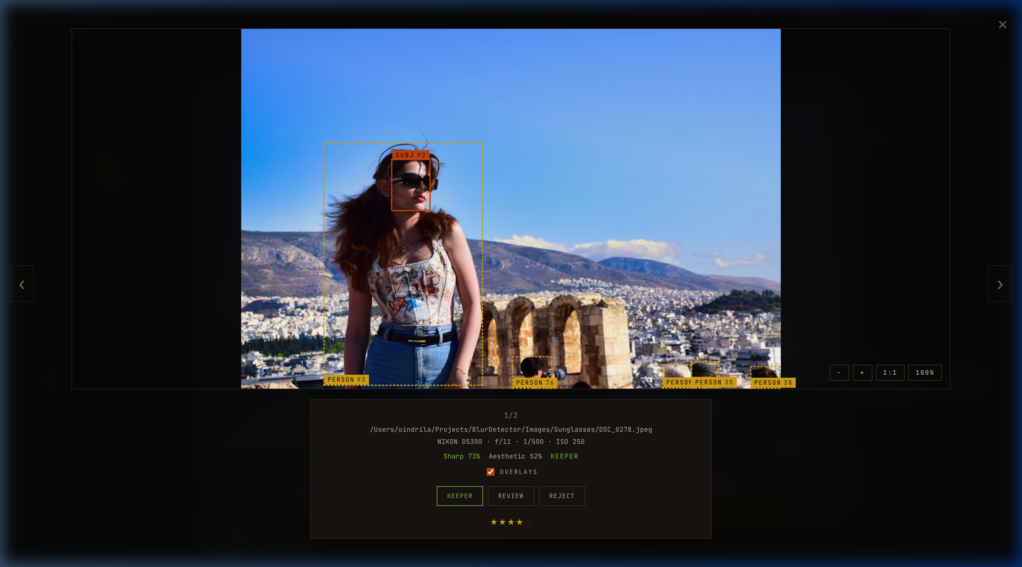 The bounding boxes the analyzer used are visible in the UI. The orange and white rectangles are the exact regions Laplacian and Tenengrad were computed on — not the full frame.
The combined score (0..1) feeds the decision engine. Below 0.30 is an automatic reject; above 0.55 is keeper-quality.
Blink Detection: Eye Aspect Ratio
Closed-eye detection uses MediaPipe FaceMesh to extract 468 facial landmarks per detected face, then computes the Eye Aspect Ratio (EAR) — vertical eye extent over horizontal. Below 0.20 indicates a closed or nearly-closed eye.
The design choice that matters: EAR is per-face, and any_closed = True if any face in the frame has a closed eye. For group portraits this is conservative on purpose — one blinking person rejects the frame. Both the threshold and the reject_closed_eyes flag are configurable.
Burst Grouping: Union-Find on Perceptual Hashes
Bursts are grouped by two criteria: perceptual hash distance (64-bit pHash, Hamming distance ≤ 10 bits) and capture timestamp proximity (within 3 seconds). A union-find merges connected components in O(N α(N)):
# snapgrade/group.py

class _UnionFind:
    def __init__(self, n: int) -> None:
        self.parent = list(range(n))

    def find(self, x: int) -> int:
        while self.parent[x] != x:
            self.parent[x] = self.parent[self.parent[x]]  # path compression
            x = self.parent[x]
        return x

    def union(self, a: int, b: int) -> None:
        ra, rb = self.find(a), self.find(b)
        if ra != rb:
            self.parent[rb] = ra
Within each burst group, frames are ranked by a weighted quality score — sharpness 45%, eye openness 20%, aesthetic 13%, exposure 12%, smile 10%, highlight clipping −10% — and the top frame is marked best_image_id. The UI filter “best-of-burst only” collapses a 600-frame event to roughly 90 candidates.
Thresholds Over Models: Why the Decision Layer Is 40 Lines
The decision engine is a pure function with no imports from the metrics layer — it takes a plain dict of metric results and a Thresholds dataclass:
# snapgrade/decide.py

@dataclass
class Thresholds:
    sharp_keeper: float = 0.55   # >= → keeper-quality sharpness
    sharp_reject: float = 0.30   # < → auto-reject
    accept_overexposed: bool = False
    accept_underexposed: bool = False
    reject_closed_eyes: bool = True
    horizon_warn_deg: float = 3.0  # warn only, never auto-rejects

    # Star score weights
    w_sharpness: float = 0.50
    w_exposure: float = 0.18
    w_eyes: float = 0.14
    w_composition: float = 0.08
    w_aesthetic: float = 0.10
Each sub-score is computed independently (exposure histogram analysis, EAR-to-score mapping, composition tilt scoring) and combined into a 0..1 quality score. Stars bin from the continuous score: ≥0.80 → 5 stars, ≥0.65 → 4 stars, and so on. Hard threshold checks come first — sharpness below sharp_reject, or reject_closed_eyes with any face blinking — so a hard reject doesn’t get softened by a strong aesthetic score.
The Thresholds dataclass serializes to JSON and lives in the database. The UI mutates it and re-classifies the whole library without touching any image file. That’s why the Settings screen feels instant:
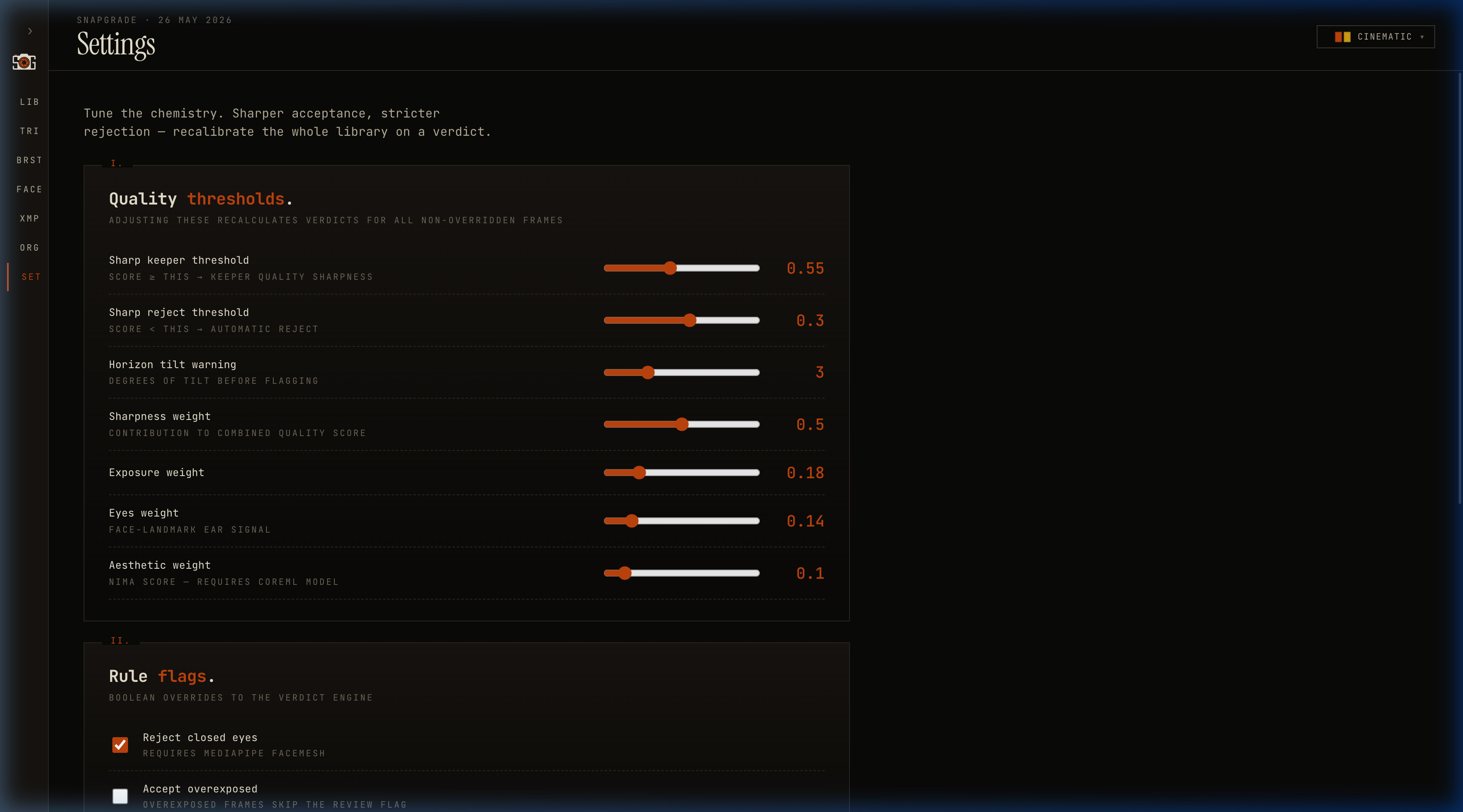 The Settings screen is a direct projection of the
 Thresholds dataclass. Moving a slider triggers a re-classification query, not a re-analysis — the metrics are already in SQLite.
The whole thing is around 40 lines of decision logic and a dataclass. A VLM call would give you a verdict and nothing to tune.
From 1.9 to 3.3 img/s: What Actually Moved the Needle
The initial pipeline ran at 1.90 img/s on 53 test images. Getting to 3.28 img/s on 2,070 images required two changes — neither in the CV.
The Decode Was the Bottleneck
Profiling showed image decoding (rawpy for RAW, Pillow for JPEG/HEIC) dominated wall time — often more than the CV inference itself. Two fixes:
- PIL draft mode. JPEGs are decoded at a reduced resolution using Pillow’s draft mode, which skips decompression work when full resolution isn’t needed for the analysis pass.
- EXIF fast path. If an embedded JPEG thumbnail exists in the RAW’s EXIF, SnapGrade uses that instead of a full RAW decode. A 1200px embedded preview is sufficient for sharpness and exposure metrics.
Thread-Local YuNet
MediaPipe and OpenCV’s YuNet face detector aren’t thread-safe across threads. The first implementation shared a single global model instance, which serialized all inference through a lock. The fix is thread-local storage so each worker initializes its own model:
_tls = threading.local()

def _get_detector() -> cv2.FaceDetectorYN:
    if not hasattr(_tls, "detector"):
        _tls.detector = cv2.FaceDetectorYN.create(...)
    return _tls.detector
Lock contention disappeared and parallel inference became real.
Numbers
| Corpus | Phase | Wall time | Throughput | Notes |
|---|---|---|---|---|
| 2,070 images | Pre-optimization | 767.6 s | 2.70 img/s | Single-threaded decode, shared model |
| 2,070 images | Post-optimization | 630.7 s | 3.28 img/s | Draft decode + thread-local models |
| 53 images | Re-run (cached) | 0.00 s | — | mtime match, zero re-processing |
The cached re-run at 58.5 MB RSS is the number I’m most satisfied with — the second pass through a library is effectively free, which matters when you’re iterating on threshold tuning.
SQLite Is the Index
All analysis results live in ~/.snapgrade/library.db. The schema uses a JSON blob column for metrics rather than individual columns — adding a metric never needs a migration, it just appears in the blob on the next analysis run. Fields are promoted to dedicated columns only when they need indexing (verdict and stars, because the UI filters on them constantly).
WAL mode is on, so read-heavy UI queries don’t block background ingest writes. The organizer, XMP writer, and report generator all read this cache — they never touch image files directly.
The payoff: the React UI is a thin client. Every filter, every threshold tweak, every burst-grouping rerun is a SQL query against cached metrics. There’s no “rebuild index” step, because the index is the database and the database is the index.
Run It Yourself
git clone https://github.com/Bibyutatsu/SnapGrade
cd SnapGrade
uv sync --all-extras

# Analyze a folder
uv run snapgrade analyze /path/to/photos

# Group bursts (loosen thresholds if your bursts are wider than 3s)
uv run snapgrade group --hamming 14 --seconds 30

# Start the API + UI
uv run snapgrade serve   # → http://127.0.0.1:8765

# Write XMP sidecars for rated images
uv run snapgrade write-xmp /path/to/photos

# Run tests
uv run pytest
The optional models — aesthetic scoring (CoreML NIMA), semantic search (MobileCLIP), face clustering (InsightFace buffalo_s), OCR, and content-type classification — are gated behind environment variables or CLI flags. The base pipeline runs without any of them.
What’s Still Open
The next significant piece is smarter subject segmentation through the already-wired subject_seg.py module — separating foreground from background should improve sharpness scoring on images with complex depth of field. There’s also an open question about whether the opt-in NIMA aesthetic model is pulling its weight relative to the compositional signals that already run unconditionally.
Source, issues, and full design rationale on GitHub: